Paper 3 · technical report · simulation study · not peer-reviewed

Algorithm for anonymous markers, reprojection filter, minimum number of frames and criterion for a successful calibration

From an anonymous T-wand to the minimum achievable error

Simone Tortorella · October 2026

Abstract

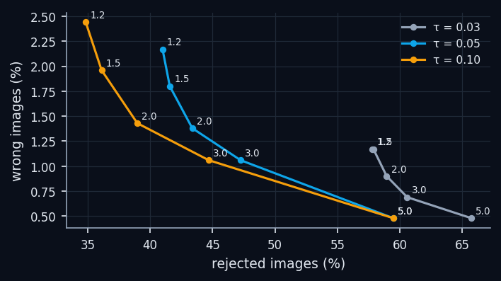
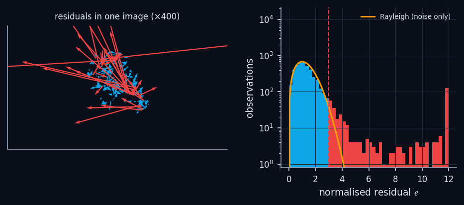
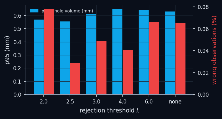
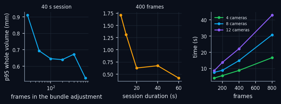
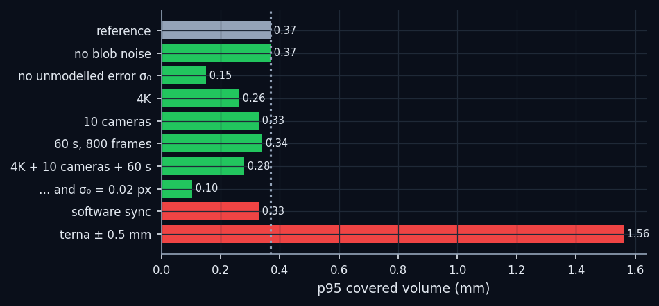
We describe and evaluate the algorithm that calibrates 8 IR monochrome cameras from anonymous blobs: T recognition by affine fit with ambiguity rejection, initial estimate from the terna, sparse bundle adjustment with rejection of observations with a high normalised residual, multi-view relabelling by Hungarian assignment, final bundle adjustment. Labelling takes 0.08 ms per image; with an ambiguity threshold of 2 it leaves 1.4% of images wrong, which relabelling reduces below 0.1% of the observations. Rejection at $k = 2.5$ –3 standard deviations is a good compromise. About 100–200 frames are enough if spread over at least 20 s of motion: duration (volume coverage) matters more than the number of frames; the bundle adjustment with 400 frames and 8 cameras takes about 15 s in Python. The reprojection residual tells good calibrations from wrong ones poorly; a validation wand (frames kept aside) does better: in 90 sessions with random defects the rule wand deviation ≤ 0.75 mm, mean deviation ≤ 0.10 mm and coverage ≥ 5% never accepts calibrations with a p95 beyond 2.9 mm, while a rule on the residual accepts some up to 10.6 mm. The error budget points to a minimum achievable error of about 0.10 mm (p95 in the covered volume, with an unmodelled centroid error of 0.02 px) and shows what limits it: the unmodelled centroid error and the terna tolerance, not blob noise.

Keywords: bundle adjustment · unlabelled markers · reprojection · outlier rejection · calibration validation · error budget

1. Introduction

Paper 1 fixed the object (asymmetric 4-marker T, 3D terna) and Paper 2 the number and placement of cameras. Here we describe the algorithm that turns anonymous blobs into a calibration, choose its thresholds using the simulation's known truth, measure what it costs in frames and time, and look for a criterion, computable without the truth, to say whether a calibration worked. Finally we build an error budget to see which minimum error can be reached and what limits it.

2. The algorithm

Algorithm 1 — calibration from anonymous blobs

Blobs: threshold at 40% of white, connected components, weighted centroid, diameter and circularity of every blob.
Terna: average of 30 frames; PnP for every camera with nominal intrinsics → initial estimate.
Per-image labelling: for every subset of 4 blobs (also dropping one as a reflection) and every permutation, affine fit to the T drawing; keep the best if $r^{*} < τ$ and every different labelling has $r > amb \cdot r^{*}$ , otherwise reject the image.
Shape filter: discard blobs that are not round or smaller than the other markers of the same image suggest (partial occlusion).
Sparse bundle adjustment (intrinsics, extrinsics, T positions, delays) with a rigidity constraint.
Rejection: remove observations with normalised residual $e > k$ ; repeat the bundle adjustment (2 times).
Multi-view relabelling: project the T estimated from all cameras into every image; assign all blobs (also of rejected images) with the Hungarian algorithm within $g$ px.
Final bundle adjustment with rejection; validation with the frames kept aside (§6).

The normalised residual of an observation $u_{c k m}$ (camera $c$ , frame $k$ , marker $m$ ) is

e_{c k m} = \frac{∥ π _{c} ( X _{k m} + δ _{c} V _{k m} ) - u _{c k m} ∥}{σ _{c k m}}, σ_{c k m}^{2} = σ_{blob}^{2} (d) + σ_{0}^{2}

(1)

where $π_{c}$ is the projection with distortion, $δ_{c}$ the camera delay, $V$ the marker velocity and $σ_{blob} (d)$ the expected centroid error for a blob of diameter $d$ (Paper 1). Relabelling solves, for every image, the assignment

ϕ min i \sum π_{c} (\hat{X}_{k, ϕ (i)}) - u_{c i} s.t. each marker used once, ∥ \cdot ∥ < g

(2)

3. Labelling: thresholds and speed

**Figure 1.** Trade-off between wrong and rejected images for the ambiguity threshold amb (numbers on the points) and the absolute threshold τ (T4a, 10% reflections, 8 cameras, 2400 images).

4. Reprojection and filtering threshold

**Figure 2.** Left: residual vectors (magnified 400 times) in one image, against the final solution; red: normalised residual beyond 3. Right: histogram of the normalised residuals of all observations (rejected ones included) of a session with 0.4% of the images containing two swapped markers; yellow: the distribution expected with Gaussian noise only (Rayleigh); the last bar collects residuals beyond 12.

Full algorithm (labelling, rejection, relabelling) versus the rejection threshold $k$: final error and share of wrong observations left. — **Figure 3.** Full algorithm (labelling, rejection, relabelling) versus the rejection threshold $k$ : final error and share of wrong observations left.

5. How many frames and how long

**Figure 4.** Left: error versus number of frames used (40 s session). Centre: versus session duration (400 frames). Right: bundle adjustment time (3 passes, Python + SciPy, one core).

6. When the calibration has worked

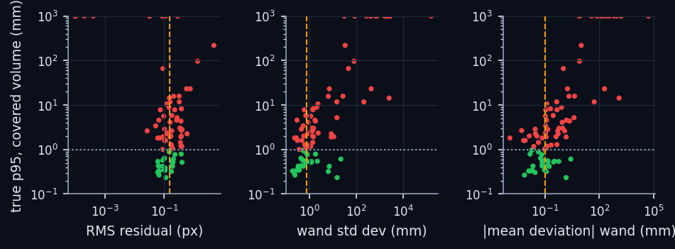
In a real installation there is no truth. We need computable quantities that predict the error. We simulated 90 sessions with random defects (few frames, short sessions, a person leaving the volume, initial focal length wrong by up to 30%, an imprecise terna, unmodelled error up to 0.3 px, up to 5% of images with swapped markers) and computed for each: the RMS reprojection residual, the coverage (share of the volume within 30 cm of a T position seen by ≥ 2 cameras), the minimum number of observations per camera and a validation wand: one frame in five does not enter the bundle adjustment and is triangulated with the estimated cameras; marker distances are compared with the known ones of the T (mean and standard deviation of the deviation). A session is "good" if the p95 in the covered volume is ≤ 1 mm.

**Figure 5.** 90 sessions with random defects: true p95 (covered volume) versus three diagnostics. Green: good (≤ 1 mm); red: not. Yellow dashed: rule thresholds.

Rule	accepted	of which good	maximum p95 among accepted
wand: dev. ≤ 0.75 mm, \|mean\| ≤ 0.10 mm, coverage ≥ 5%	20	13	2.9 mm
residual ≤ 0.15 px, coverage ≥ 5%	29	14	10.6 mm

Table 1. The two rules on the 90 sessions (27 good).

The wand rule also accepts a few calibrations above 1 mm, but never beyond 2.9 mm; the residual rule accepts some up to 10.6 mm. In practice the wand should be used as an error estimate rather than a yes/no test: the 95th percentile of the wand deviations has a correlation of 0.70 (log scale) with the true error, the residual 0.49. An independent check is even better: a second wand of known length moved through the whole volume after calibration, because the validation frames here come from the same trajectory as the calibration and do not see the regions the T never crossed.

7. Error budget and feasibility

To see which minimum error can be reached we start from the reference configuration (8 Full HD cameras at two heights, 60 fps, 20 s, 30 mm markers, hardware trigger) and remove or improve one error source at a time.

**Figure 6.** Error budget: p95 in the covered volume removing or improving one source at a time (median of 4 sessions). Green: improvements; red: degradations.

Sensitivity to the unmodelled centroid error $\sigma_0$ (8 Full HD cameras). — **Figure 7.** Sensitivity to the unmodelled centroid error $σ_{0}$ (8 Full HD cameras).

Parameter	Effect	How to lower it
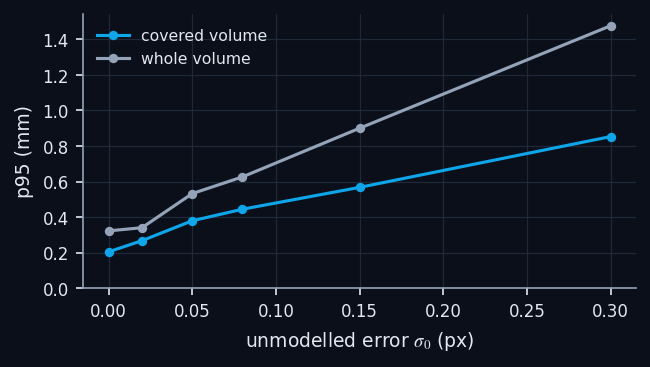
Unmodelled error $σ_{0}$	dominant; ~linear	richer distortion model, global shutter, rigid mounts, thermal stabilisation
Terna tolerance	dominant on absolute accuracy	terna machined to 0.1 mm or measured with a CMM arm
Synchronisation	×4–6 over the volume	hardware trigger
Partial occlusion	bias ∝ diameter	small markers, shape filter, 3σ rejection
Volume coverage	error outside the covered volume	40–60 s sessions guided by a live coverage map
Resolution / number of cameras	secondary for calibration	4K if markers must be small

Table 2. Feasibility: what limits the error and what can be done to lower it further.

8. Conclusions

Algorithm, thresholds, minimum error

Labelling: affine fit over every assignment, amb = 2, τ = 0.05; no tracking (it propagates errors).
Filters: shape (circularity ≥ 0.93, diameter ≥ 0.9 × the expected one) and rejection at $k = 2.5$ –3 of the normalised residual.
Multi-view relabelling within 6 px (Full HD) before the final bundle adjustment.
Session: ≥ 20 s (better 40–60 s), 100–400 frames; T seen by ≥ 2–3 cameras together.
Criterion: validation wand with deviation ≤ 0.75 mm and mean deviation ≤ 0.10 mm, coverage ≥ 5% (never accepted calibrations beyond 2.9 mm); better still, a second wand moved through the whole volume. The reprojection residual alone is not enough.
Minimum achievable error in simulation ~0.10 mm (p95, covered volume); in practice limited by $σ_{0}$ and the terna.

Limits: thresholds were chosen on simulated data with known truth; on a real system they must be checked with an independent measuring object (for example a second wand of known length). The 90 sessions of the criterion cover plausible defects but not all (for example cameras knocked during the session).

References

B. Triggs, P. McLauchlan, R. Hartley, A. Fitzgibbon, Bundle adjustment — a modern synthesis, LNCS 1883, 2000.
H. W. Kuhn, The Hungarian method for the assignment problem, Naval Research Logistics Quarterly 2, 1955.
R. Hartley, A. Zisserman, Multiple View Geometry in Computer Vision, 2nd ed., 2004.
M. A. Fischler, R. C. Bolles, Random sample consensus, Communications of the ACM 24(6), 1981.
W. Kabsch, A solution for the best rotation to relate two sets of vectors, Acta Crystallographica A32, 1976.