3D reconstruction of anonymous markers with unknown mutual distances
Epipolar correspondences, multi-view consensus and tracking
Simone Tortorella · October 2026
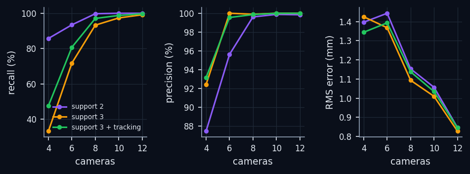
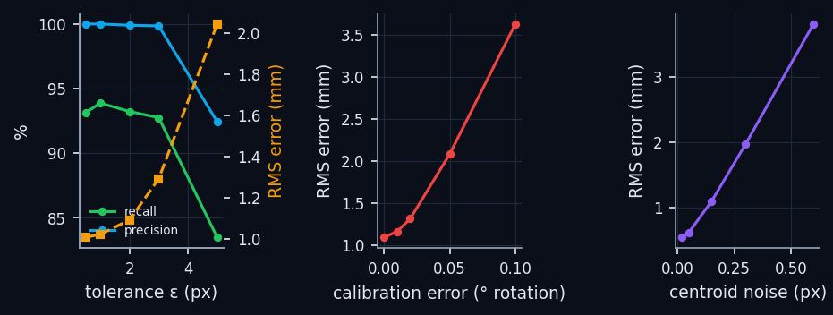
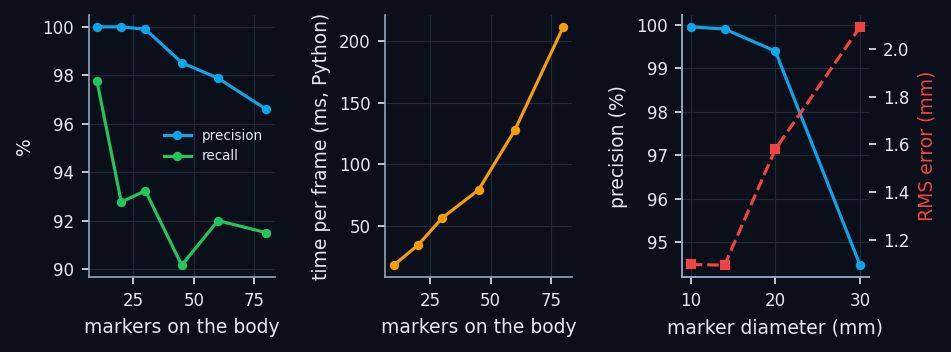
After calibration, the markers on an athlete's body must be reconstructed in 3D without knowing which blob corresponds to which marker and without knowing the distances between markers (they are not on a rigid object). We propose a four-step algorithm: candidate correspondences along the epipolar lines between camera pairs, counting each candidate's support in the other cameras, greedy selection with the "one blob, one point" constraint and refinement, constant-velocity 3D tracking. In simulation (30 14 mm markers on a walking person, 8 Full HD cameras, 0.15 px noise, reflections) the algorithm reconstructs 97.0% of the markers seen by at least two cameras with 99.9% precision and an RMS error of 1.14 mm, in 59 ms per frame in Python. Recall depends mostly on the number of cameras (it converges between 8 and 10), the error on the calibration and on the centroid noise: 0.05° of camera rotation error doubles the 3D error. The best epipolar tolerance is 1–2 px. Finally we describe how to implement it in real time.
Keywords: unlabelled markers · epipolar geometry · multi-view triangulation · correspondences · 3D tracking
1. The problem
Papers 1–3 calibrate the cameras with a rigid object whose marker distances are known. On the athlete this is not the case: markers are attached to skin or clothes, distances change with motion and are not known in advance. Each camera sees anonymous blobs; some markers are hidden by the body, two nearby markers can merge into one blob, reflections add blobs that correspond to nothing. The task is to find the 3D positions of the markers using only the calibration, with no body model.
The difficulty is combinatorial: with cameras and blobs per camera there are combinations of correspondences. Two rays from different cameras also come close by chance: an intersection of only two rays can be a ghost point. Epipolar geometry reduces the candidates, the consensus of several cameras confirms them.
2. Simulated scene
A person walks (1.4 m/s) or runs (3 m/s) through the 3.5×3.5×2 m volume. The body is made of capsules (trunk, head, upper arms, forearms, thighs, shanks, feet) moving with a gait cycle; spherical 14 mm markers are spread at random over the capsules, fixed to the segment. For each camera: a marker is visible if the ray from the camera does not cross any capsule; two markers whose image distance is smaller than the sum of their apparent radii produce a single blob at their midpoint; each image receives 0.3 reflections on average; centroids have 0.15 px Gaussian noise. The cameras are the 8 of Paper 2 (two height rows, Full HD, 120° lenses). Each configuration is simulated for 40 frames at 60 fps.
3. Algorithm
For two cameras , with relative rotation and translation , a 3D point seen in normalised coordinates and (undistorted) satisfies the epipolar constraint
The distance of a blob from the epipolar line is ; multiplied by the focal length it is in pixels and is compared with the tolerance .
- Undistort all blobs (normalised coordinates).
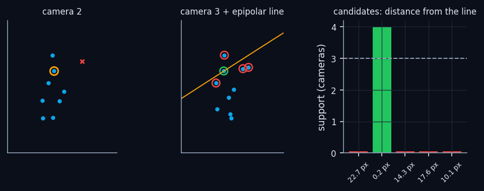
- For every camera pair and every blob of : blobs of within px of the epipolar line are candidates; triangulate each candidate pair (DLT).
- Support: project every candidate into all other cameras and add the nearest blob if within px.
- Sort candidates by decreasing support and increasing residual.
- For each candidate: drop views whose blobs are already used; if at least views remain ( if a track predicts it nearby), re-triangulate with all views (DLT + 3 Gauss–Newton steps on pixels), check the residuals (< 1.5 ), discard duplicates within 8 mm, mark the blobs as used.
- Tracking: associate points with tracks (constant velocity, Hungarian assignment within 4 cm); a point is confirmed after 2 frames; a track survives 3 frames without observations.
The cost is dominated by the candidates: epipolar tests and projections for the support, with candidates. The "one blob, one point" rule is what removes ghosts: a chance intersection of two rays rarely finds support in a third camera, and if its blobs are already explained by a point with more support it is discarded.
4. Results
The metrics are: recall (share of markers seen by at least 2 cameras reconstructed within 1 cm), precision (share of reconstructed points that correspond to a true marker: 1 − ghosts), RMS error of the right points and time per frame (Python + NumPy, one core).
| Configuration | Recall | RMS error (mm) |
|---|---|---|
| HD | 92,6 | 1,67 |
| Full HD | 93,2 | 1,09 |
| 4K | 93,8 | 0,61 |
| walking, 8 cameras | 97,0 | 1,14 |
| running, 8 cameras | 88,7 | 1,23 |
| running, 10 cameras | 89,8 | 1,10 |
| 3 reflections per image | 93,4 | 1,08 |
Resolution reduces the error in proportion to the pixels (the noise in pixels is fixed): 0.61 mm in 4K against 1.67 mm in HD. In running recall drops a few points because constant-velocity tracking struggles with the feet (abrupt velocity changes) and occlusions are shorter but more frequent; with 10 cameras it recovers only in part. Reflections, even 3 per image, do no harm: they find no support.
5. How to implement it
The Python reference implementation takes ~59 ms per frame with 8 cameras and 30 markers: fine for offline analysis, not for real time at 120 fps (8.3 ms per frame). The plan for real time:
| Module | Where | What it does | Cost |
|---|---|---|---|
| Blobs | camera or edge box | threshold, connected components, centroid, diameter, circularity; sends only blobs (≈ 1 kB/frame) | < 1 ms (FPGA/GPU) |
| Synchronisation | server | aligns frames by trigger timestamp (or estimated delays) | — |
| Epipolar candidates | server | for each pair, sorts blobs along epipolar lines (1D index) instead of testing all: | 0,2 ms |
| Support and selection | server (GPU) | vectorised projections, sorting, greedy selection | 0,5 ms |
| Refinement | server | DLT + 3×3 Gauss–Newton per point | 0,1 ms |
| Tracking | server | constant-velocity Kalman, 3D Hungarian | 0,1 ms |
| Labelling | server | assignment of points to the body model (outside this paper) | — |
From the calibration we need intrinsics, distortion and extrinsics of each camera and, if cameras have no hardware trigger, the estimated delay (preliminary study). During use, two indicators show whether the calibration has degraded (a camera knocked, thermal expansion): the mean residual of the accepted points per camera and the share of each camera's blobs that do not enter any point. If a camera exceeds the thresholds, only that camera is recalibrated with the T.
6. Conclusions
- Epipolar correspondences + support in other cameras + "one blob, one point" rule: reconstructs anonymous markers without knowing distances and without a body model.
- 8 cameras, support 3 and tracking: recall 97.0%, precision 99.9%, error 1.14 mm RMS.
- Parameters: ε = 1–2 px, support 3 (2 with a track), tracking gate 4 cm (6 cm when running).
- Accuracy is set by calibration and centroid noise; recall by the number of cameras.
- Real time: blobs on the cameras, candidates with an epipolar index, selection on GPU: < 2 ms per frame estimated.
Limits: capsule body, randomly placed markers, no skin-sliding model; the next step is assigning the 3D points to a body model (3D labelling), not treated here.
References
- R. Hartley, A. Zisserman, Multiple View Geometry in Computer Vision, 2nd ed., 2004 (geometria epipolare, triangolazione).
- H. W. Kuhn, The Hungarian method for the assignment problem, Naval Research Logistics Quarterly 2, 1955.
- R. E. Kalman, A new approach to linear filtering and prediction problems, J. Basic Engineering 82, 1960.
- M. A. Fischler, R. C. Bolles, Random sample consensus, Communications of the ACM 24(6), 1981.
- S. Tortorella, Paper 1–3, calibrazione con marker IR anonimi, 2026.